Equivalence of Linear State-Space and Autoregressive Models
Recent works such as the S4 paper and the Hyena Heirarchy, have brought to light (to the ML world) the equivalence of linear state-space models and convolution models. Here, we explore the correspondence between state-sapce models and autoregressive models. This relationship can be understood via algebraic manipulations of a shift operator.
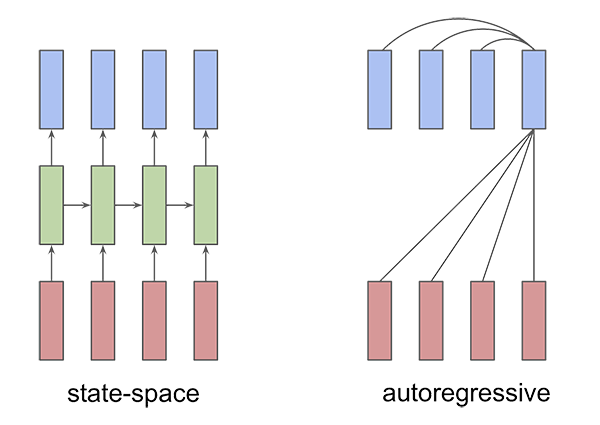
State-Space Model
A linear discrete-time state-space model is represented by:
\begin{align} x(t+1) &= Ax(t) + Bu(t) \\ y(t) &= Cx(t) + Du(t) \end{align}
where $u\in\mathbb{R}^m$ is the input, $x\in\mathbb{R}^n$ is the state, and $y\in\mathbb{R}^p$ is the output. The matrices $A, B, C,$ and $D$ are of compatible dimensions.
Autoregressive Model
An $n$-th order autoregressive model expresses the current output $y(t)$ as a function of the past $n$ outputs, and past-and-current inputs $u(t)$, formulated as:
\begin{align} y(t) = \sum_{i=1}^n \alpha_iy(t-i) + \sum_{j=0}^n \beta_ju(t-j) \end{align}
with $\alpha_i\in\mathbb{R}^{p\times p}$ and $\beta_j\in\mathbb{R}^{p\times m}$. Note that the indices $i$ and $j$ range differently.
This is sometimes called an ARX model (autoregressive with external inputs).
Conversion: From State-Space to Autoregressive
The goal is to convert state-space equations to ARX equations.
Step 1: Rewrite State-Space Equations in Terms of Shift Operator
The shift operator $q$ advances a signal by one time step, so $qx(t) = x(t+1)$. Using $q$ as a variable, the state-space equations become:
\begin{align} x(t) &= (qI-A)^{-1}Bu(t) \end{align}
The output equation is:
\begin{align} y(t) &= \left(C(qI-A)^{-1}B + D \right)u(t) \\ y(t) &= H(q)u(t) \end{align}
where $H(q)$ is the transfer function. This derivation is valid if $(qI-A)^{-1}$ (an operator) is boundedly invertible and if $u(t)$ is bounded for all $t$.
Step 2: Express $H(q)$ as a function of $q$
The transfer function $H(q)$ includes an inverse term $(qI-A)^{-1}$. A matrix inverse is a ratio of its adjugate and determinant. By utilizing this property we have,
\begin{equation} H(q) = \frac{C\operatorname{adj}(qI-A)B + D\operatorname{det}(qI-A)}{\operatorname{det}(qI-A)} \end{equation}
By applying the adjugate and determinant formulas, each entry of the matrix $H(q)$ can be shown to be a quotient of polynomials of $q$. The degree of each polynomial is at most $n$ and the degree of the numerator is less than or equal to the degree of the denominator (a proper rational function of $q$).
Step 3: Re-arrange to Obtain Autoregressive Form
Each entry of $H(q)$ shares the same denominator but different numerators. For notational simplicity we assume $p=m=1$ (single-input, single-output). We can now re-arrange and apply higher-order shifts $q^i$s to obtain the autoregressive equation as:
\begin{align} y(t+n) = \sum_{i=0}^n f_iu(t+i) - \sum_{j=1}^{n-1}g_jy(t+j) \end{align}
The coefficients $f_i,g_j\in\mathbb{R}$ can be expressed in terms of the state-space parameters $A,B,C,D$ (again, via application of the adjugate and determinant formulas).
Conversion: From Autoregressive to State-Space
Converting an autoregressive model to a state-space model is called the realization problem. Since we can apply similarity transforms to the state without affecting input-output behavior we know that there are infinitely many realizations of a given autoregressive model. One can choose a canonical realization.
Relation to Z-Transform
The discrete-time analog of the Laplace transform is the Z-transform, which converts a time-domain signal to a function in the complex number domain. The Z-transform of a shifted signal is represented as $\mathcal{Z}(x(t+1)) = zX(z)$. The entire derivation process above can be redone with $z$ in place of $q$, yielding $Y(z) = H(z)U(z)$, where $H(z)$ is also the transfer function.
References
[1] Verhaegen, M., & Verdult, V. (2007). Filtering and system identification: A least squares approach. Cambridge University Press.