Spelling Out the Equivalence of RNNs, CNNs, and Autoregressive Models in the Linear Case
This note spells out the equivalence of convolution, state-space, and autoregressive architectures for linear dynamical systems. This is a well-known exercise in engineering but less-known in machine learning. This exercise may be useful for improving intuition of sequence modeling in general, and for making sense of the RNN vs CNN vs AR architecture debates in ML.
We have a sequence of inputs $u(t)\in\mathbb{R}^m$ and outputs $y(t)\in\mathbb{R}^p$ indexed by time $t\in\mathbb{Z}$.
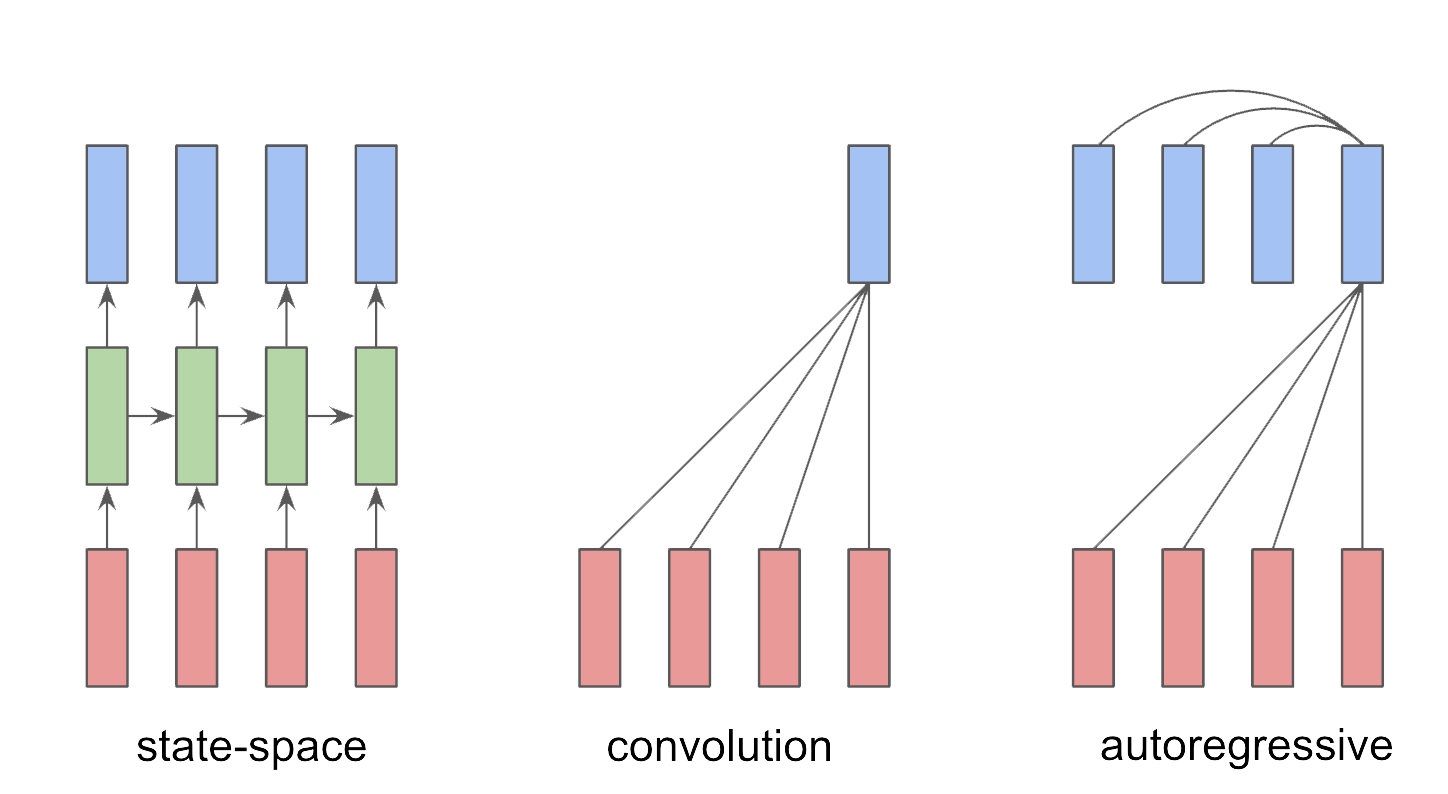
There are three main architectures for modeling of the current $y(t)$.
- Convolutional: $y(t)$ depends on current and past inputs $u(t), u(t-1), u(t-2), \dots$
- Autoregressive: $y(t)$ depends on past outputs $y(t-1), y(t-2), \dots, y(t-T)$
- State-space: $y(t)$ depends on state variable $x(t)$ which in turn depends only on current input $u(t)$ and previous state $x(t-1)$.
When these arechitectures are linear they become effectively interchangeable, despite appearances.
The six LTI Representations
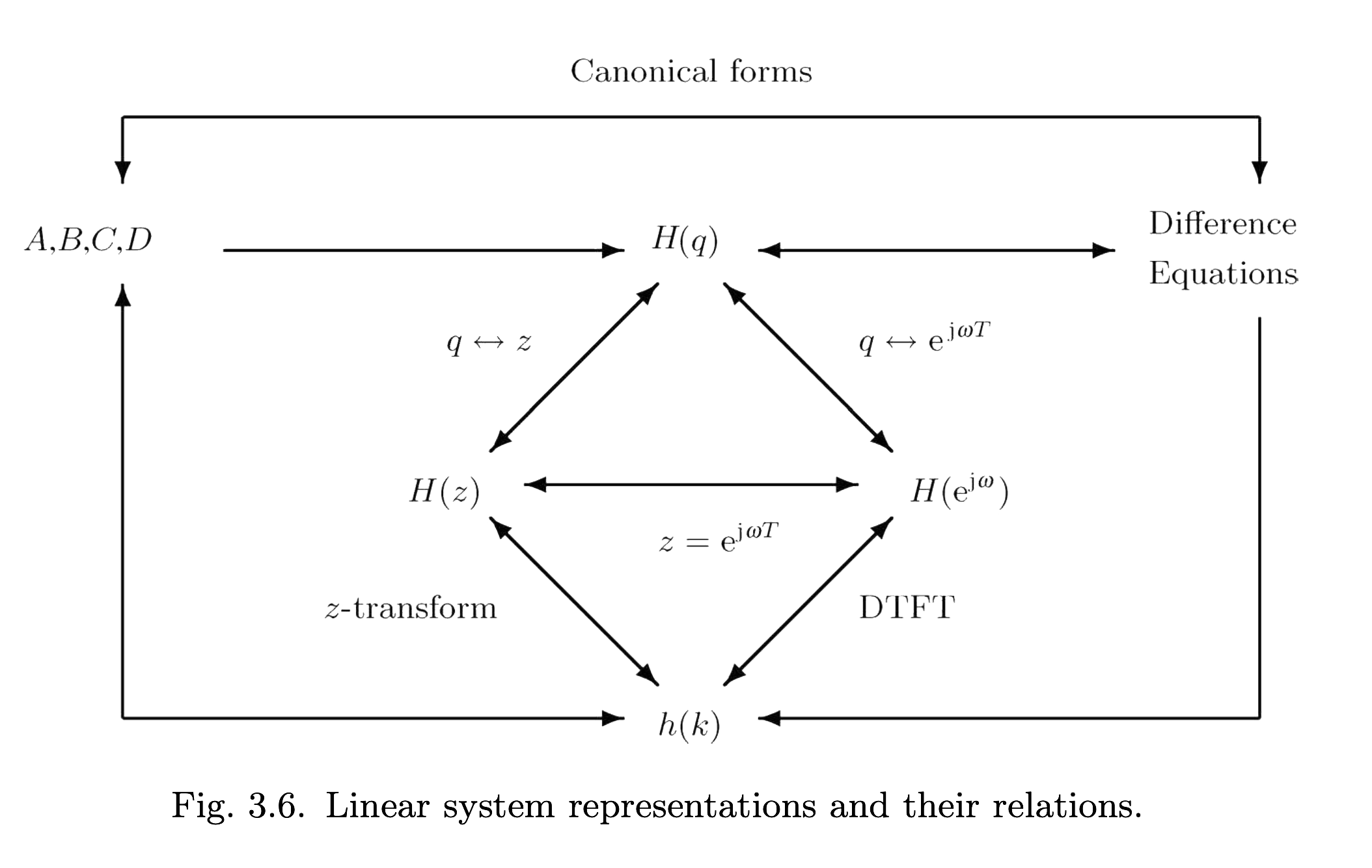
To be consistent with the engineering literature on LTI systems, and for completeness, we’ll go through six representations of a discrete-time linear time-invariant system (figure from [1]).
Architecture representations:
- State-space (aka linear RNN)
- Convolution (aka impulse-response)
- Autoregressive (aka difference equations)
Transfer Function representations:
- Transfer function $H(q)$ of shift operator $q$
- $z$-Transform transfer function $H(z)$ of complex variable $z$
- DTFT transfer function $H(\omega)$ of complex variable $\omega$
The transfer function representations are essentially different viewpoints of the autoregressive representation. They’re a bit more abstract, but are still heavily emphasized in engineering texts.
Let’s go through defining each representation, and along the way build the machinery for converting between them.
1. State-space
It’s easiest to start with the state-space (SS) representation.
The SS representation is parametrized by matrices $A,B,C,D$. A.k.a. a linear RNN,
\begin{align} x(t+1) = Ax(t) + Bu(t) \\ y(t) = Cx(t) + Du(t) \end{align}
2. Convolution
The convolution (or impulse-response) representation is given by \begin{align} y(t) & = h(t) \ast u(t) \ & = \sum_{j=t}^{\infty} h(i) u(t-i) \end{align}
Where $\ast$ represents a discrete convolution and $h(t)$ is a $p\times m$ matrix that varies with $t$.
From SS $\rightarrow$ Conv
Given a state-space representation, we convert to a convolution representation by assuming a zero initial state $x(0) = 0$. This amounts to solving the recurrance equation (unrolling the SS model) and obtaining, \begin{align} y(t) = \sum_{i=1}^\infty CA^{i-1} B u(t-i) + Du(t), \end{align} which implies convolution parameters, \begin{align} h(t) = \begin{cases} D & t=0 \\ CA^{t-1}B & t \geq 1. \end{cases} \end{align}
The convolution has infinite receptive field but finite parameters – the “weights” are parametrized by $t$. In the case that $A$ is nilpotent then $h(t)$ does go to zero for large enough $t$ thus giving a finite receptive field but this is not common.
3. Autoregressive
We set $p=m=1$ in the following for notational compactness. The autoregressive representation is \begin{align} y(t) = \sum_{i=1}^n a_i y(t-i) + \sum_{i=0}^n b_i u(t-i) \end{align}
where $a_i, b_i \in\mathbb{R}$. (An autonomous autoregressive model has no input terms.)
The current output $y(t)$ depends on the past $n$ outputs. Wherease the state-space representations contains only first-order differences, the autoregressive representation is expressed in higher-order differences.
Unlike in the convolutional model, there are finite terms here. The upper index $n$ is intentional notation – it turns out that when an $n$th order autoregressive model is converted to a state-space model we need an $n$-dimensional state vector.
4. Transfer function $H(q)$ of shift operator $q$
We can rewrite the autoregressive equation in a slightly clever way. We turn (discrete) calculus into algebra. The shift operator $q$ shifts a signal as in $qx(t) = x(t+1)$. And $q^i$ shifts $i$ times. The shift operator is the discrete-time analog of the continuous-time derivative operator. So, we can simply write
\begin{align} y(t) - \sum_{i=1}^n a_i y(t-i) &= \sum_{i=0}^n b_i u(t-i) \\ r(q)y(t) &= s(q)u(t) \end{align} where $r(q) = (1 - a_1 q - \dots - a_n q^n)$ and $s(q) = (b_0 + b_1 q + \dots + b_n q^n)$ are polynomials in $q$. And if we divide both sides by $r(q)$ we obtain \begin{align} y(t) = H(q)u(t) \end{align}
where $H(q) = \frac{s(q)}{r(q)}$ is the transfer function in $q$.
For $m>1, p>1$, $H(q)$ is a $p\times m$ matrix, each entry of which is a rational function of $q$.
This is kinda of nice. We turned (discrete) calculus (difference equations) into algebra. There should be some lingering questions around whether we can just treat an operator $q$ as if it were an algebraic variable. For this, there is some extra rigor needed but I defer to ([1]).
From SS $\rightarrow$ $H(q)$ $\rightarrow$ Autoregressive
Now for a fun part. Given an SS model we can turn it into $H(q)$, and if we have $H(q)$ we can just multiply the denominator polynomial on both sides, distribute the $q^i$ terms as shifts, resulting in the AR model.
We first specify the SS equations with $q$ and treat $q$ as an algebraic variable. \begin{align} qx(t) &= Ax(t) + Bu(t) \\ x(t) &= (qI - A)^{-1} Bu(t) \\ \end{align} with output equation \begin{align} y(t) &= (C(qI - A)^{-1} B + D)u(t) \\ y(t) &= H(q) u(t) \end{align}
The key observation is that matrix inverses such as $(qI - A)^{-1}$ can be written as $(qI-A)^{-1}=\frac{\text{adj}(qI-A)}{\text{det}(qI-A)}$, which imply both numerator and denominator reduce to polynomials of $q$ of degree at most $n$. And exact values of the polynomial coefficients can be derived (painstakingly) from the adjugate and determinant of the matrix $qI-A$. We then can write out the full $H(q)=C(qI-A)^{-1} B + D$, where each entry of the matrix is a proper rational function of $q$. Each entry shares the same denominator polynomial, but different numerator polynomials.
It follows that $H(q)=C(qI-A)^{-1} B + D$ is a proper rational function of $q$. In the $p=m=1$ case, we write \begin{align} H(q) = \frac{b_n q^n + \dots + b_1 q + b_0}{a_n q^n + \dots + a_1 q + a_0} \end{align}
Given that $H(q)$ is a proper rational function of $q$, we can multiply both sides of $y(t) = H(q)u(t)$ by the denominator polynomial and apply shift operators $q^i$ to obtain the autoregressive representation.
From SS $\rightarrow$ H(q) $\rightarrow$ convolution
We already derived the convolution representation above. But let’s derive it from $H(q)$.
We can also note that the $(qI-A)^{-1}$ is the resolvent of $A$ (but with $q$ instead of a complex variable). Reminding ourselves of geometric series, we can expand $(qI-A)^{-1}$ into an infinite series \begin{align} (qI-A)^{-1} &= q(I - q^{-1}A)^{-1} \\ &= \sum_{i=0}^\infty q^{-i} A^i \end{align} (Since $q$ is an operator this is really a Neumann series). Since each $q^{-i}$ applies $i$ negative shifts, we can rewrite the transfer function representaiton as \begin{align} y(t) = H(q)u(t) y(t) = \sum_{i=1}^\infty CA^{i-1} B u(t-i) + Du(t) \end{align}
which is consistent with the convolution representation from section 2. above, but it’s interesting to see the $h(t)$ parameters emerge from a different angle.
5. Transfer function $H(z)$ of complex variable $z$
Most engineering textbooks omit the $H(q)$ representation and instead approach it from a slightly different viewpoint using the $z$-transform instead of $q$. The steps are essentially identical due to how the $z$-transform acts on shifts.
If we apply the $z$-transform to the state-space equation we obtain \begin{align} X(z) = (zI - A)^{-1} BU(z) \end{align} where $X(z)$ and $U(z)$ are the $z$-transforms of $x(t)$ and $u(t)$.
We get \begin{align} Y(z) &= (C(zI - A)^{-1} B + D)U(z) \\ &= H(z) U(z) \end{align}
Which is identical to the $H(q)$ but with complex variable $z$ in place of shift operator $q$.
6. DTFT representation
For completeness we note that we can also take the DTFT \begin{align} Y(\omega) = H(\omega) U(\omega) \end{align} Where $Y(\omega)$ is the DTFT of $y(t)$ and is related to the $z$-transform via $z = e^{i\omega T}$. This allows us to define the frequency response of the system.
Realization, from $H(q)$ to SS
Everything so far was done by starting with SS parameters.
If we start with either an autoregressive or convolution model, we can convert to an SS model. This is called realization. This is generally more involved but revolves around the construction of a Hankel matrix.
Assume we are given the convolution parameters $h(t)$ and construct the Hankel matrix: \begin{align} \mathcal{H} = \begin{bmatrix} h(0) & h(1) & h(2) & \dots & h(n-1) \\ h(1) & h(2) & h(3) & \dots & h(n) \\ \vdots & \vdots & \vdots & \ddots & \vdots \\ h(n-1) & h(n) & h(n+1) & \dots & h(2n-2) \end{bmatrix} \end{align}
We assume that $\mathcal{H}$ decomposes as
\begin{align} \mathcal{H} = \begin{bmatrix} C \\ CA \\ \vdots \\ CA^{n-1} \end{bmatrix} \begin{bmatrix} B & AB & \dots & A^{n-1}B \end{bmatrix} \end{align}
The rank of $\mathcal{H}$ will be equal to $n$, the state dimension. So by taking the SVD of $\mathcal{H}$ we “read out” the $A,B,C$ matrices from the (top $n$) left singular vectors and (top $n$) right singular vectors accordingly. This defines system matrices up to a similarity transformation.
If instead we are given an autoregressive model we can take its corresponding proper rational function into an infinite series to obtain the convolution parameters $h(t)$ then construct the Hankel matrix.
We omitted many details, but this is the general idea. Realization is a large topic.
Summary
We intentionally omit some details and rigor. The point is to give a scaffolding of these connections. The texts [1], [2], and [3] provide the best exposition on this topic that I’ve been able to find. The setup here is mostly inspired by [1]. Stanford’s EE263 is also an excellent course for learning about LTI systems.
Everything here is in discrete time. The continuous time case is analogous, with the Laplace transform taking place of the Z transform.
References
[1] Verhaegen, M., & Verdult, V. (2007). Filtering and system identification: A least squares approach. Cambridge University Press.
[2] Antsaklis, P. J., & Michel, A. N. (2007). A linear systems primer. Springer Science & Business Media.
[3] Antoulas, A. C. (2005). Approximation of large-scale dynamical systems. Society for Industrial and Applied Mathematics.